What is group cohomology?

Of all the ubiquitous and mysterious algebraic tools that appear in number theory and arithmetic geometry – and surely, there are many – group cohomology remained an impenetrable black box to me for quite a while. Although I still consider myself a near absolute beginner in the topic, my goal in this post is to demystify it at least a little for those unfamiliar with it and hoping to get a window into its inner life.

The window through which we will peak is called Galois descent.

First, I’m going to to explain by example the type of glimpse I want to give. If you’ve ever studied any algebraic topology, you’re surely familiar with the singular cohomology of a topological space, and you also likely know that the cohomological cup product gives these groups (collectively) the structure of a graded-commutative ring. What you may not know, however, is that when the modern definition of cohomology was first formulated in the mid-1920’s, mathematicians like Schubert and Poincaré had already been computing these rings for more than half a century!

So how were they studying cohomology before cohomology existed? The answer is called the intersection ring. Consider a closed smooth manifold, and think about the free abelian group on the set of all closed submanifolds. We can define a natural equivalence relation by identifying submanifolds that can be wiggled onto eachother. (More precisely, we use cobordism: kill off a linear combination of submanifolds if their disjoint union is the boundary of a submanifold – not necessarily closed – in higher dimension.) Finally, we can define a product by wiggling pairs of submanifolds until they intersect transversally, and then taking intersections. This gives us a graded-commutative ring, where the grading is by codimension.

Now if we triangulate all the submanifolds in the picture, we can turn them into simplicial chains. In fact, the relation of cobordism turns out to be exactly equivalence-mod-boundaries, and the group we constructed is exactly the direct sum of singular homology groups! Better yet, since we’re on a closed manifold, we can use Poincaré duality to move the ring structure to cohomology, and there it miraculously agrees with the regular old cup product! This alternative intersection-ring description of the cohomology ring has a narrower definition (it doesn’t work on arbitrary topological spaces), but it has much richer geometric intuition, and it was the object of interest to the 19th century geometers mentioned above.

My goal here is less ambitious, but it has a similar flavor. Group cohomology is an invariant of a group acting on another group. In a very, very special case (in the case of a Galois group acting on the automorphism group of one of a few types of interesting object) I want to give an explicit and concrete description of the first cohomology of this action. We’ll finish up by using this description to give a wonderfully simple proof of Hilbert’s theorem 90, which I claim essentially just says that all one-dimensional vector spaces are isomorphic!

What is Galois descent?

Galois descent studies the following hilariously vague problem: let k be a field, probably not algebraically closed, and let X be a thing over k. It might be:

1. An algebraic variety, maybe a plane conic, for instance.
2. A vector space.
3. An algebra.
4. More generally, we could consider a vector space equipped with some other kind of extra linear structure, such as a linear or bilinear form. (Note that an algebra is a special case of this; it’s just a vector space with a bilinear form satisfying some identities.)

Pretty much anything goes, provided that it has one important property: we need to be able to “tensor” with field extensions, to move our object X to bigger fields. In cases 2-4, it’s obvious what we mean: a literal tensor product of vector spaces. In case 1, it’s also not too bad: tensor product just means regular old algebraic geometry base change. (Take the same equations and put them over a bigger field!)

In general, we’ll write  or  for this base change when L/k is the field extension.

Galois descent attempts to answer the following question: given a field extension L/k and an L-thing X, which k-things become isomorphic to X when we tensor everything with L? In other words, when is ? These are called the Galois twists or just twists of X.

When our extension is a separable closure, and X is the projective line, we are classifying plane conics up to isomorphism. When X is a matrix algebra, it is a (very nontrivial) fact that the objects Y are precisely the central simple k-algebras of the same dimension, and the theory presented here is the first step in describing the Brauer group of a field in terms of cohomology.

(In fact, with the right formalism, the examples of a matrix algebra and a projective space are basically the same!)

For a general extension, this is a hard problem, but when the extension L/k is Galois, we can exploit the Galois group in a fabulously cool way.

Actually doing descent

First, let’s set up some notation.

1.  is the Galois group of our field extension.
2. is the group of automorphisms of our object X.

The surprising goal of the next couple paragraphs is to construct a map

. 

Then, we’ll modify the target of this map to get a bijection, and find out that the set on the left can be naturally thought of as a cohomology set!

So how does this map work? Well we obviously need to start with some suitable Y, and then we need to choose an isomorphism . (For now, our map will depend on this choice. We’ll fix that later.) Additionally, we need some , and we need to explain where it goes in . To do this, notice that an automorphism of the field extension induces an automorphism of and one of .

Beware: these automorphisms are weird! In particular, suppose  is a real vector space and our field extension is . Then complex conjugation acts on , but it is not a -linear map; it’s only -linear! This is something to be aware of, but it won’t be an issue, in the end.

Now we have maps  and , and together with our original isomorphism f, we get a square diagram of maps. But lo! This diagram does not commute! Of course, when we have a square diagram of isomorphisms, its failure to commute is measured by a particular automorphism of any one of the objects present – we’ll pick X. The point is that if we start at X and work around the square, composing as we go, we’ll get an automorphism – an element of A, just like we wanted! So our map is given by

,

where exponentiation denotes conjugation, to simplify the notation: .

Note that we kept the isomorphism f as part of our notation, since the map isn’t quite well-defined on Y alone, yet. We’ll fix this soon. The rest of what we want to do will now be summarized as a series of exercises, some easy and some hard, and the interested reader is encouraged to try them all out!

From this point on, we’ll forget about case 1, where X is an algebraic variety. While this is an important and interesting case of descent, it is harder, and the statements are not as simple and explicit as what we’re about to prove. So now let’s take X to be a vector space, possibly with some additional linear structure.

Exercises

1. In your favorite case of our construction (variety, vector space, algebra, etc.), check that this the map  really lands in the automorphism group. That is, check that even though  and  are only k-linear, the whole composite described above is actually L-linear.
2. Verify the identity

   

   Such a map is called a twisted homomorphism, and we’ll denote the set of these maps by .

3. Consider any twisted homomorphism . Produce some Y/k which becomes isomorphic to X over L (by some isomorphism f, for instance), and with the property that . (Try to give an operation of G on X using your map, although it won’t quite be a group action. Now check that the subspace of invariants is a k-subspace – with whatever linear structure you imposed – and that the inclusion becomes an isomorphism when we pass back to L.)
   We now have a “surjection” (which is still not yet well-defined)

   .

4. Next, consider another isomorphism . The composite map  is an automorphism of X. Verify that the  and  are related by the formula

   .

   Now if we let ~ denote the equivalence relation that we’ve just described, we have a well-defined surjection

   .

5. Finally, check that this map is injective by proving the converse to 4: if two twisted homomorphisms are related as in 4 by some automorphism , then they in fact come from the same k-object Y, just with a different choice of isomorphism .

So the moral is this: objects that become X after a base change along L/k (provided L/k is Galois) are the same thing as twisted homomorphisms  up to some equivalence relation. Let’s call that latter set .

While it may not be obvious whether this thing is any easier to compute than what we started with, it’s pretty easy to see that these sets, when A is abelian, have a natural group structure, and are really Ext-groups, which can be studied with all the machinery of homological algebra. When A is not abelian, the picture is not as nice, but often we can understand them by fitting A into short exact sequences with abelian groups, and then studying long exact sequences. (Details of all this can be found in any number of books, such as Serre’s Local Fields, the appendix to Silverman’s Arithmetic of Elliptic Curves, and Cassels and Froelich’s Algebraic Number Theory.)

We conclude with a final application, which will apply these ideas “in reverse,” computing a cohomology group by a trivial observation about base change. This theorem is commonly referred to as Hilbert’s theorem 90. If you’ve taken a basic graduate field theory or number theory class, you may have seen a form of this result, although you might be surprised by how easy the proof is using the observations here!

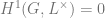
Theorem Let L/k be a Galois extension of fields with Galois group G. Then

.

Proof  The group is the automorphism group of a 1-dimensional L-vector space (with no extra linear structure). The k-vector spaces V with  are really just the one-dimensional ones, and those are all isomorphic! Therefore, this cohomology set has only one element. 

This fact, which may seem esoteric right now, can be combined with the long-exact group cohomology sequence to give an extremely easy proof of the main result of Kummer theory, which totally classifies cyclic extensions of fields with enough roots of unity. The results of Kummer theory are essentially the model and inspiration for class field theory, which is also typically proven using group cohomology.

Exercise  Note that . Generalize this proof to any ! In fact, the same proof works for n an infinite cardinal.

I’ll end with a question about something that I suspect is probably well-studied, but that I certainly know nothing about. Essentially, the goal of representation is to relate arbitrary groups to linear groups like the ones whose cohomology we’ve just come to understand, and this begs the following question:

• Under what circumstances does a subgroup of a linear group consist of the automorphisms of some linear structure?
• Can we do this systematically, and find canonical linear structures associated to a wide class of groups, particularly linear structures whose twists are easy to understand?